Output Data Review

We are currently reviewing the MERRA File Specification Document, and considering new variables and diagnostics that should be incorporated into future experiments and reanalyses. This is directed toward information that needs to be captured during run time, as opposed to diagnostics that can be post processed from existing data. For example, to get Max/Min temperature from MERRA would be the maximum/minimum hourly averaged temperature, in the current configuration. We will implement for future analyses hourly maximum and hourly minimum temperatures, so that the instantaneous Max/Min T can be captured from the system.

Any suggestions would be welcome. Please include any computations that may be non standard, and reasons or applications of the suggested diagnostic.

Apologies for letting the blog become stagnant. While I have seen a lot of interesting work with reanalyses and MERRA, finding the time to work up a worthwhile post is remarkably challenging.

Extrapolation to P > Ps

As many have found, MERRA pressure level data does not provide values for pressure surfaces when they are greater than the surface pressure (e.g. high topography).  Other reanalyses extrapolate the data using the surface meteorology and assumed lapse rates. This data may be useful in some cases such as zonal averaging, stream functions and thickness calculations.

A recent post at reanalysis.org provides user developed codes to fill these undefined grid points. This should be useful as one could adapt the codes to the filling method applied in other reanalyses to better match their extrapolated data.

See Extrapolation of MERRA Reanalyses to obtain continuous fields for more information.

Return of the MERRA Blog

As many readers will understand, the demands on time can be many, and there is never enough time to do all that you want to do. Being spread thin for some time, the MERRA blog fell into neglect. However, with a lot of interesting things going on, from research with MERRA to formulating plans for subsequent reanalyses (and noticing in the last month a fair number of hits from around the world), I will be trying hard to find time to make regular posts.

The original purpose of the blog was to 1) follow the development of the MERRA system and eventually the production of data and then 2) follow the research that was being done with MERRA and other reanalyses. #2 never fully materialized, but there is a lot of work being published on reanalyses lately.  So, for the near future, summaries of published research or perhaps topical discussions involving several papers/reports will likely be the regular topic. However, new reanalysis development is on the horizon, as well.

Mostly, I figure that the hits on the MERRA blog are coming from internet searches for hard to find information, now that the MERRA overview paper is printed. This is an important issue, as users need to know if a reanalysis is applicable to a research topic, and its strengths and weaknesses. So, perhaps this can open the communication, just a little more.

Ancillary Land and Ocean data

Two data sets for Ocean and Land have been released through the GES DISC, derived from MERRA, but not included in the original data collection. The ocean data has 1 hourly fluxes, meteorology and stresses over both open water and ice. the MERRA-Land data is an offline reprocessing using MERRA atmospheric forcing with bias corrected precipitation to produce a new set of surface fluxes and land states (Reichle et al. 2011).

See the release page for more information.

MERRA Special Collection

Papers are now available at the AMS Online Journals MERRA Special Collection. The MERRA Overview by Rienecker et al. should be considered as the fundamental citation for the MERRA project and data set.

Update to Data Streams

We are updating MERRA data to permit longer spinup of streams 2 and 3. The announcement and how it affects data downloads follows. Data files formally available in the MERRA data streams are being renamed "SPINUP_*" and will also be available for download. Most research and applications for the data will only require use of the "Mainstream" MERRA data.

Updating of the MERRA data products site to contain only Mainstream data (http://disc.sci.gsfc.nasa.gov/mdisc/data-holdings/merra-mainstream-and-spinup-data) will begin Thursday, March 11, 2010. A two step procedure will be followed to achieve this. In step one, all current  products for the years 1989 through 1992 and 1998 through 2000 will be deleted. It is strongly advised that the MERRA data for the two aforementioned periods not be accessed until this data update is complete.  In step two,  
 products will be used to repopulate these data years. We anticipate that it will take about two weeks to complete the data update. The remaining year
s of the data and all the MERRA data services will still be available during this time period. Once the update activities are completed, a new notification will be sent out and posted on the web. We thank you for your patience during this period.  If you have any questions or concerns please send an email to the GES DISC User Services (help-disc@listserv.gsfc.nasa.gov).


So when the update is complete, Stream 1 will contain 1979 through 1992, Stream 2 will have 5 years spinup (4 available for download) containing 1993 through 2000, and stream 3 will have 4 years spinup (3 available for download) containing 2001 through present.

2009 data should become available during the week of March 15.

Pressure levels greater than surface pressure

Some questions have come in regarding differences between MERRA and other reanalysis at pressure 1000mb and 850mb pressure levels. It is very important to note that MERRA does not extrapolate pressure level data vertically greater than the surface pressure. The result is that there is undefined data points in much of the 1000mb fields. This will affect the representativeness of both time and area averages of MERRA data compared with reanalyses or other data that extrapolates gridpoints to pressure levels greater than the surface pressure. The GMAO provides a summary of the impact that this has on averaging. In addition, the FAQ will be updated to call out this difference with other data sets. The main GMAO www page also has other pages with useful practical information about the data and assimilation system.

Main stream and spinup data

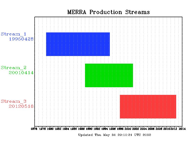
The original plan for MERRA production was to run in three streams, optimizing the computers processes. The original three streams were 1) 1979-1988, 2) 1989-1997 and 3) 1998-present. These were initialized with 2 years of coarse resolution analysis, followed by 1 year at the native (1/2 degree) resolution. Recently, streams 1 and 2 caught up to the beginning of the respective subsequent streams, connecting the time series. Streams 1 and 2 were continued providing overlapping data with the beginning of the next streams, in order to test the variance of the system and the viability of the initialization. At present, each of the overlapping periods are now 3 years duration (1989-1991, and 1998-2000).

We have been evaluating the initial conditions and the continued spinup of streams 2 and 3. In general, there are few differences in the meteorology between the overlapping data. In fluxes (such as precipitation), we do not a small difference at the beginning which gets smaller in time. The differences would likely not affect any scientific results. Slightly larger differences can be seen in slowly varying states, such as the root zone wetness.

At present we are documenting these differences and will provide a report on the overlapping period. In the mean time, this letter is provided to users to alert them that we will be changing the transition times of the streams to utilize the additional data produced at the ends of stream 1 and 2. This does not invalidate the data currently available, but is considered only a minor scientific revision. Once the data is provided to the DAAC and prepared for user access, the new streams and transitions will be as follows:

• Stream 1 1979-1991
• Stream 2 1992-2000
• Stream 3 2001-present

Connecting these streams will be presented to users as the primary MERRA data, or the “main stream” data. Access to Stream 2 1989-1991 and Stream 3 1998-2000 data will still be provided, but the data will be considered secondary and called “spinup” data. This will effectively increase the spinup period for Streams 2 and 3 to 4 years of native resolution analysis.

We anticipate the transition from the original streams to this extended spinup configuration to occur in February 2010, nearly coincident with Stream 3 catching up to real time. Regular updates on this will be made after the holidays.

Have a wonderful Holiday Break!!

Katrina Quick Look

In looking at some land hydrology in the southern US, a question came up on the effect of the 2005 hurricane season on the hydrology time series. So, we started looking around at the evolution of Katrina. This animation shows the MERRA version of Katrina (13Mb gif) moving over the southern tip of Florida and through the Gulf of Mexico. The colors show precipitation in mm/day and the white contours are sea level pressure (contour interval 2mb). The Best Track location is plotted every six hours. Firstly, the MERRA closed low pressure follows the best track fairly well throughout the evolution. This is notable only in that while MERRA does assimilate observations every six hours, there is no relocating or bogusing routines involved with the analysis/forecast cycles.

The MERRA resolution (1/2 degree) is not fine enough to get at the mesoscale structures in hurricanes, and we see that in MERRA where the surface winds (not shown) only reach Category 2 on the Saffir-Simpson scale (observations and estimates of Category 5 occurred during Katrina). Likewise, the rainbands at a distance from the central low are not well defined. The animation shows a curious shift of the main rain fall from the southern quadrant to the north, as landfall occurs (see also the figure below). In trying to validate this, we found radar data at NCDC, presented is in the second plot below, which agrees with the MERRA distribution. However, and also likely related to the resolvable scales in the MERRA grid, the heaviest precipitation in MERRA is a larger distance away from the central low than observed.

While this seems like it is a reasonable representation of the real system, and likely useful, users must consider carefully the limitations in MERRA or any reanalysis data set when applying it to a project.

Figure 1. MERRA precipitation (color, mm/day) and sea level pressure (mb) at 12Z29AUG2005 with the complete NHC best track path for Hurricane Katrina.

Figure 2 Nexrad radar rainfall at 12:32Z29AUG2005.

Hurricane Andrew, Aug 1992

MERRA Stream 2 has completed through 1993. We have been looking at various weather and climate events. Hurricane Andrew was a powerful, but fairly small hurricane. MERRA's 1/2 degree resolution is likely too coarse to adequately resolve the circulation, and there is no bogus or center relocation being done in the system. Still, assimilation of observations will show some circulation or feature.

There isn't much of a circulation prior to landfall in Southern Florida. Landfall was at 9Z24Aug1992. Figure 1 shows the sea level pressure and wind barbs from 6Z the closest analysis time before landfall. The pressure center is much higher than the observed center pressure (955 mb). the center of the pressure is located south of the best track at that time. The feature that really attracted attention is the offset of the wind circulation, even further south than the pressure center, and crossing the isobars at the center.

Figure 1 MERRA Sea Level Pressure and 1000 mb wind barbs from the 6Z 24 AUG92 analysis. The blue line shows the best track befre and after landfall, with red markers at 00Zs.

A closer look at the observations being assimilated shows that ERS1 did track over the center of circulation around 6Z. Figure 2 shows all the observations accepted into the analysis. There are ERS1 wind vectors crossing the center of the circulation, and the assimilation system accepted the data. The vectors closest the center are likely contaminated by precipitation, and should have been rejected. At this point, it's not clear how often this kind of problem occurs, or what might be done to detect and reject the bad data. It's under investigation.
An important point for reanalysis users, especially as resolutions are increased to better resolve weather and smaller scale circulations, is that reanalyses are assimilating vast quantities of observations. sometimes poor quality data does make it into the analyses. While quality of data and analyses are improving, users still need to consider that features may or may not be realistic. Likewise, we are providing some information on the accepted observations in MERRA. More difficult is providing access to the users on the actual observations.

Figure 2. MERRA analysis sea level pressure, analysis streamlines and windbarbs showing the accepted observations (red is buoy or ship, black is ERS1). Most of the ERS1 vectors seem to agree with the mass field, however, close to the center of the low pressure the ERS1 vectors are crossing the isobars. The wind analysis is drawing to the observations, even when they disagree with the mass field.

Incremental Analysis Update

GEOS5 uses an Incremental Analysis Update (IAU) to constrain the atmospheric numerical model by observations. The following figure shows the schematic of the procedure. Starting at 09Z, a 6 hour forecast is run, and forecast data from 09Z, 12Z and 15Z are used to create the analysis (blue diamond). From the analysis and the forecast, a tendency is calculated. This tendency is applied to another model forecast cycle in the prognostic equations (green arrow and light blue box). This is called the corrector segment, so that the tendencies are nudging the model forecast in the direction of the observations at every time step.

MERRA will have two primary products. First, the analyses will consist of the model state variables written instantaneously after the analysis every 6 hours (00Z, 06Z, 12Z and 18Z). There will be model level (72 eta levels) and pressure interpolated (42 pressure levels) for each analysis time. Second, the diagnostic fields are written from the model corrector segment. These include 1 hourly average 2 dimensional (1/2 deg latitude by 2/3 degree longitude) surface, single level (e.g. H500), radiation, land specific and vertically integrated fields. In addition, 3 hourly average 3 dimensional coarse resolution 1.25 deg x 1.25 degree) atmospheric diagnostics are produced from the corrector segment. These include all the tendencies for the state variables, as well as fluxes and budget terms.



One advantage of IAU is that it allows the corrector segment data to be written. This data is exposed to the observational forcing spread out in time, rather than a large change in the initial conditions. The spin up spin down problems in the forecast, associated with initializing a forecast system with an analysis data, are much smaller. Essentially, this allows the production of 1 hourly precipitation and other physics fields. The figure below shows a global average precipitation time series (data is written at every model time step, ~30 min) using the synoptic analysis as initial conditions, IAU and a pure model forecast. Reinitializing the forecasts with the analysis causes jumps in the time series. The free running model tries to have a global precipitation rate of ~3 mm/day. The analysis tried to reduce that, but after the initial time the forecast starts to drift back to it's preferred climate state. The IAU provides forcing at every time step, constraining the system with the observations.

Pressure levels intersecting the surface

Many modern atmospheric numerical models use terrain following vertical coordinates, meaning that the pressure of the lowest model level tracks the topography and does not intersect the surface. ERA40 and NCEP reanalyses have produced pressure level data extrapolated downward beneath the Earth’s surface. The result is that for 850, 925 and 1000 mb levels etc, continuous grids are available. Previous versions of GEOS models and assimilation systems have not extrapolated data beneath the surface, favoring to provide undefined values when the surface pressure is lower than a given pressure level.

For instantaneous analyses, comparing GEOS5 pressure levels to other reanalyses would be straight forward, once the undefined value is considered. However, monthly averages pose a problem. There are some regions and pressure levels where the number of valid values may be available for a fraction of the times. If all valid values of GEOS5 are averaged and reported, the average would not be representative or comparable to NCEP or ERA40 reanalyses which made averages of all times.

Figure 1 850 mb temperature RMS error between GOES5 and NCEP analyses for different criteria of the sampling of missing data in the GEOS5 time series. At the left of the graphs, lower criteria allow undersampling of the monthly time series to be compared with NCEP complete monthly mean. Far right, rejects points that have missing data in the time series, so there are fewer data points, but the comparisons to NCEP are more completely sampled. (Click figure to enlarge)

This can lead to an increase in the squared error and systematic bias between GEOS5 and other reanalyses because of the temporal sampling at the edges of topography. This is also noticeable in global and regional map comparisons. We computed global monthly averages testing a range of criteria for rejecting a monthly average. The criteria are applied at each grid point and are based on the percentage of valid data over the month. In Figure 1, on the far left, if data are valid only 1% of the time during a month, a valid monthly mean value is saved. Moving right, at 20%, a grid point with valid data 20% of the month produce a monthly mean (fewer than 20% are reported as undefined). At the farthest right, the strictest criteria requires that for each gridbox to produce a monthly average much have gridpoints that have valid data 100% of the time. The two figures are global land only and North America (20-70, -170--60). At higher pressure, there are more points affected by sub-sampling, and the errors are most noticeable in these large area averages. For higher altitudes, the large scale error drops slowly for criteria greater than 20% (more points valid 100% of the time).

Figure 2 Comparison between GEOS5 and NCEP for different criteria, and a map of the sampling percentage. At 20% criteria (data is valid only 20% of the month) large differences are apparent. These are reduced at 80%. At 100% the data should be showing only differences between full monthly averages, no effect of sampling. There are some artifacts because these figures have interpolated NCEP to the GEOS5 ½ degree resolution. Differences near topography can be significant and misleading (to one not knowing about the character of the data). (Click figure to enlarge)

To address this issue in the monthly mean MERRA products, only means which include counts that exceed a threshold of 20% valid data are included in the mean. Otherwise, the monthly mean value is reported as undefined. This low value is defined to provide as much information as possible. The monthly mean 3D pressure files will also include a variable that counts the valid data at each pressure level. The data user can then screen data to suit their needs. This can also be used to screen other data sets for comparison purposes, and also zonal averaging.

One difficulty that may arise is the lack of a 1000-500 mb thickness diagnostic. This was produced in some previous versions of GEOS5. However, in revising the pressure level interpolation code for MERRA, the calculation of 1000 mb height has been left out, and so, 1000-500 mb height is not available. Also, consider that the 1000 mb analyses will have undefined data over large areas of the globe (land and ocean). Lowest model level data are also available that may be suitable for some purposes, instead of the 1000mb level.

Land Fractions

One feature in the GEOS5 GCM that is different previous reanalyses is fractional surface tiles, as opposed to a land/sea mask. Each grid box contains a fraction of land, water, lake or land ice. The fractions are based on the 1km Global Land Cover Characteristics (GLCC) database. Along coast lines, the land processes are blended with sea surface processes. Inland, lakes and rivers are also included. This will require some attention of users calculating precise budgets. For example, the grid box average evaporation that would be appropriate for an atmospheric budget, may not be appropriate for in-situ data comparisons and land surface budget studies, if the lake fraction is substantial. Figures showing some examples of land and lake fractions are shown below.

To support the analysis of land water and energy budgets, a land only output data collection will be produced (tavg1_2d_lnd_Nx in the MERRA File Specification Document). These grids would be for the land only fraction of the surface. Users will be able to differentiate land evaporation from total evaporation in grid boxes near the coast and near inland water bodies. Soil water (GWET variables) will show up in grid boxes that appear to be oceanic. The model does provide an integer land/ocean mask (variable name LWI). However, this is simply a 50% cutoff between land/land ice and ocean fractions. For some specific purposes, this may not be appropriate, and users should use the land fraction to develop their own mask.

Additionally, the land fraction is subset into tiles based on the Catchment hydrology. The land collection includes data from the catchments. For more information, the interested reader should review Koster et al. (2001, J. Geophys. Res. Vol. 105 , No. D20 , p. 24,809, 2000JD900327).

Upcoming Runs and Plans

An update to the file spec was posted on the MERRA WWW page this week. No major changes, but it is still a draft.

We fully expect to have the system ready for production by mid-July. As such we are gearing up for the validation runs. The reanalysis system is also being configured for the new Discover super computing system. This provides a significant performance increase. A new partition for MERRA is being prepared.

The runs will be:

Jan/Jul 2001, Pre-AIRS period where we have legacy experiments, including the GEOS4 validation

Jan-Apr and Jul-Oct 2004: We want a full annual cycle, but that will take a substantial amount of time to run. As a shortcut, we'll run two experiments that will provide the central month of the four seasons, so most focus will be on Jan, Jul then Apr, Oct. This should show any red flags that might require us to hold production. However, we plan to keep the Jan 2004 run going beyond April, as computing cycles permit, with the idea that we will get a full annual cycle (the start of production will not be held up for that to finish, but we will evaluate it nonetheless).

Jan 2006: We have been using this case for several experiments so far, and have some familiarity with it.

We have been formulating a list of comparisons and issues to consider in validation. I'll post that separately in a couple days.

MERRA Introduction

NASA's Modern Era Retrospective-analysis for Research and Applications (MERRA) is intended to be a full reanalysis of the satellite era. In general, the data provided will support science research and applications.

The official MERRA WWW site is: http://gmao.gsfc.nasa.gov/merra/

This Blog is intended to be an interface between the developers and user community, and a place for status updates and Q&A regarding the MERRA production and data.